 Ruby
Ruby
 Golang
 .Net
.Net
 MCP
MCP
 C++
C++

This week we'll talk about how to implement ML on Rails using torch.rb, torchtext-ruby, and gruff in detail.
Changes in procedure this week:
- Dumping of maximum word size (can be found on #1 of the blog post series)
Creating Dataset
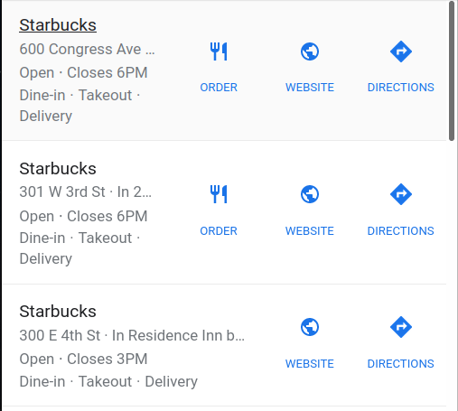
Before we start how we created a custom dataset using SerpApi engines, let me clarify one point. Google Local Pack Results are given or taken the same kind as Google Local Results.
Former shows itself in the organic search results page (without using any extra parameters). But they represent the same thing. Their key fields are also the same. So we can train a model for classifying ingredients of Google Local Results, and then use it for Google Local Pack Results.
We decided to use a rake function to create our custom datasets. For that we’ll use a preset JSON file we will parse and then fill using SerpApi.
{
  "local_results": {
    "title": [],
    "place_id_search": [],
    "thumbnail": [],
    "rating": [],
    "reviews": [],
    "type": [],
    "phone": [],
    "address": [],
    "hours": [],
    "price": [],
    "description": [],
    "place_id": [],
    "lsig": []
  },
  "queries": [
    "McDonald’s",
    "Starbucks",
    "Subway",
    ...
  ],
  "params": "engine=google&tbm=lcl",
  "query_parameter": "q"
}
local_results here represents the type of results, all the keys within it are different keys we extract in Google Local Results.
queries is a set of queries to create the dataset. In this case it contains famous restaurants and coffeehouses in the US.
params are relevant parameters in a normal SerpApi Search.
query_parameter represents the parameter key to be used in the search.
Rake command will use the path of the JSON file as an argument to fill it with the relevant data. Each result we get from SerpApi will be checked if its key names are the same as key names within the JSON and then it’ll be added inside the dataset.
Here is an example for Google Local Result and Playground link for the example:
Loading the Data
We need to create some class variables to be used within the custom data loader and pass some of them to the trainer.
    def initialize(json_file_path)
      super()
      @@all_letters = []
      @@data = File.read(json_file_path)
      @@data.split('').each {|letter| (@@all_letters << letter) unless @@all_letters.include? letter}
      @@n_letters = @@all_letters.size
    end
@@all_letters is filled with each unique character within the JSON file. This is helpful for creating an index for different kinds of data which we will come in a second.
@@data is the JSON hash of the file we read.
@@n_letters is our dictionary size. It’ll be the size of every unique character used to create our results.
We also need a way to get back our dictionary, and dictionary size in the training module:
    def self.declare_dictionary
      return @@all_letters, @@n_letters
    end
In order to avoid reading and writing issues with special characters, we need to transform them to Unicode:
    def self.to_unicode string
      I18n.transliterate string
    end
We need only the necessary parts we want to extract from @@data to work with it:
    def self.read_from_json
      data = JSON.parse(@@data)
      data = data[data.keys.first]
      data
    end
Each letter needs to be indexed within the dictionary (or alphabet, I use them interchangeably in this context) before we transform them into tensors.
    def self.letter_to_index letter
      letter = to_unicode(letter)
      @@all_letters.find_index letter
    end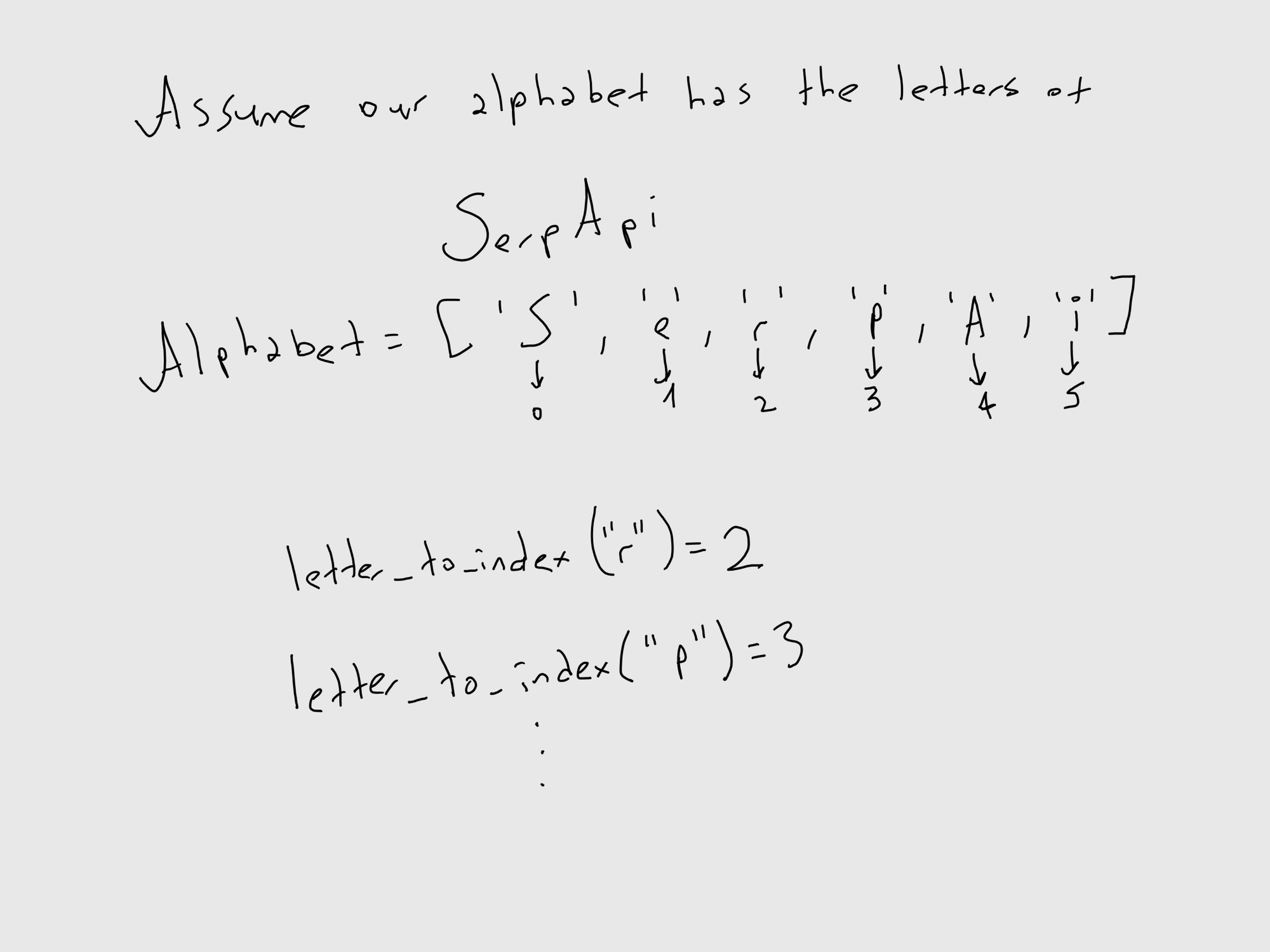
From there we make tensors out of them with the size (1 x @@n_letters):
    def self.letter_to_tensor letter
      tensor = Torch.zeros(1, @@n_letters)
      tensor[0][letter_to_index(letter)] = 1
      tensor
    end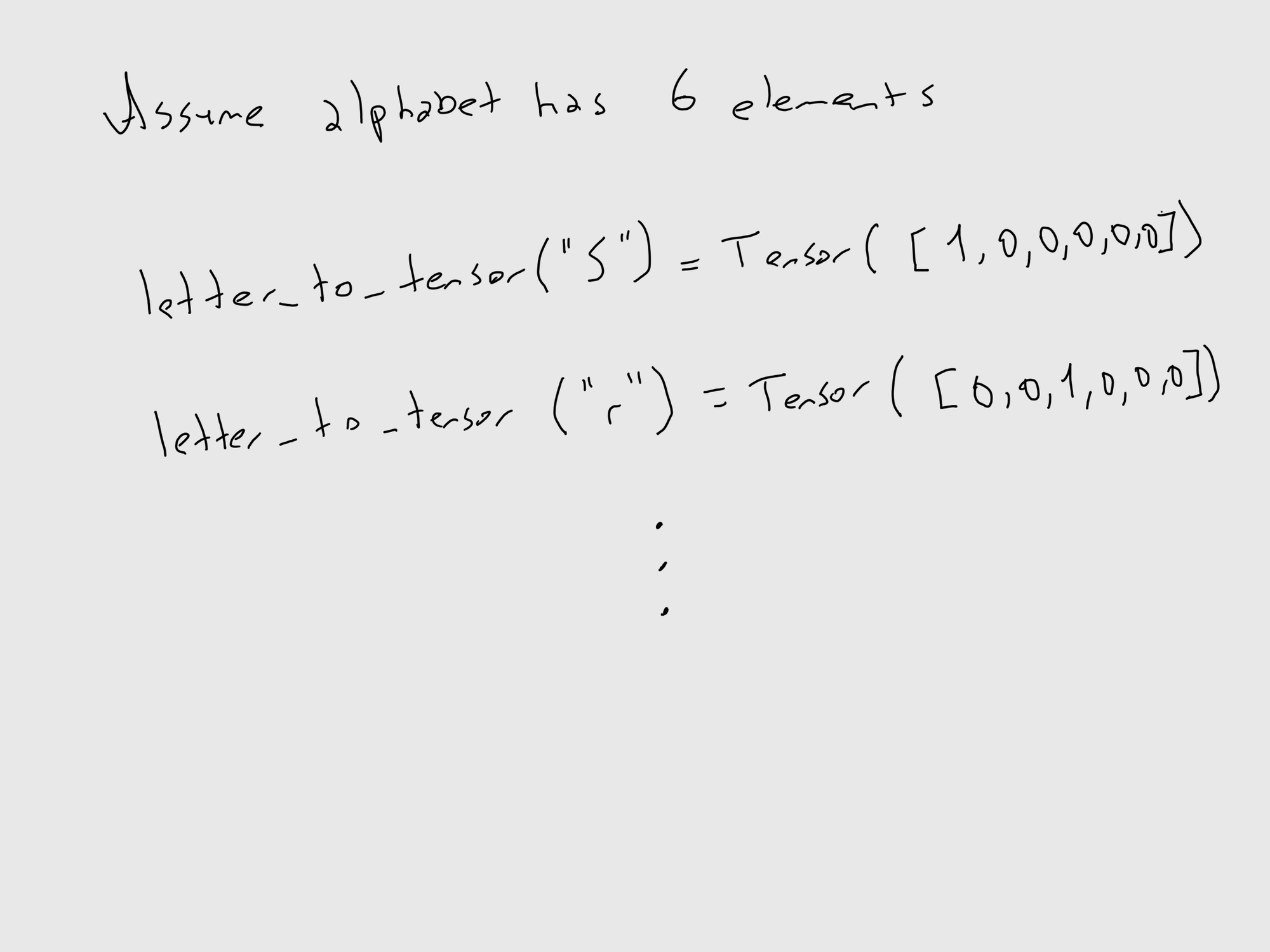
Thus each word will be consisting of letter tensors:
    def self.word_to_tensor word
      tensor = Torch.zeros(word.size, 1, @@n_letters)
      word.split('').each_with_index do |letter, index|
        tensor[index][0][letter_to_index(letter)] = 1
      end
      tensor
    end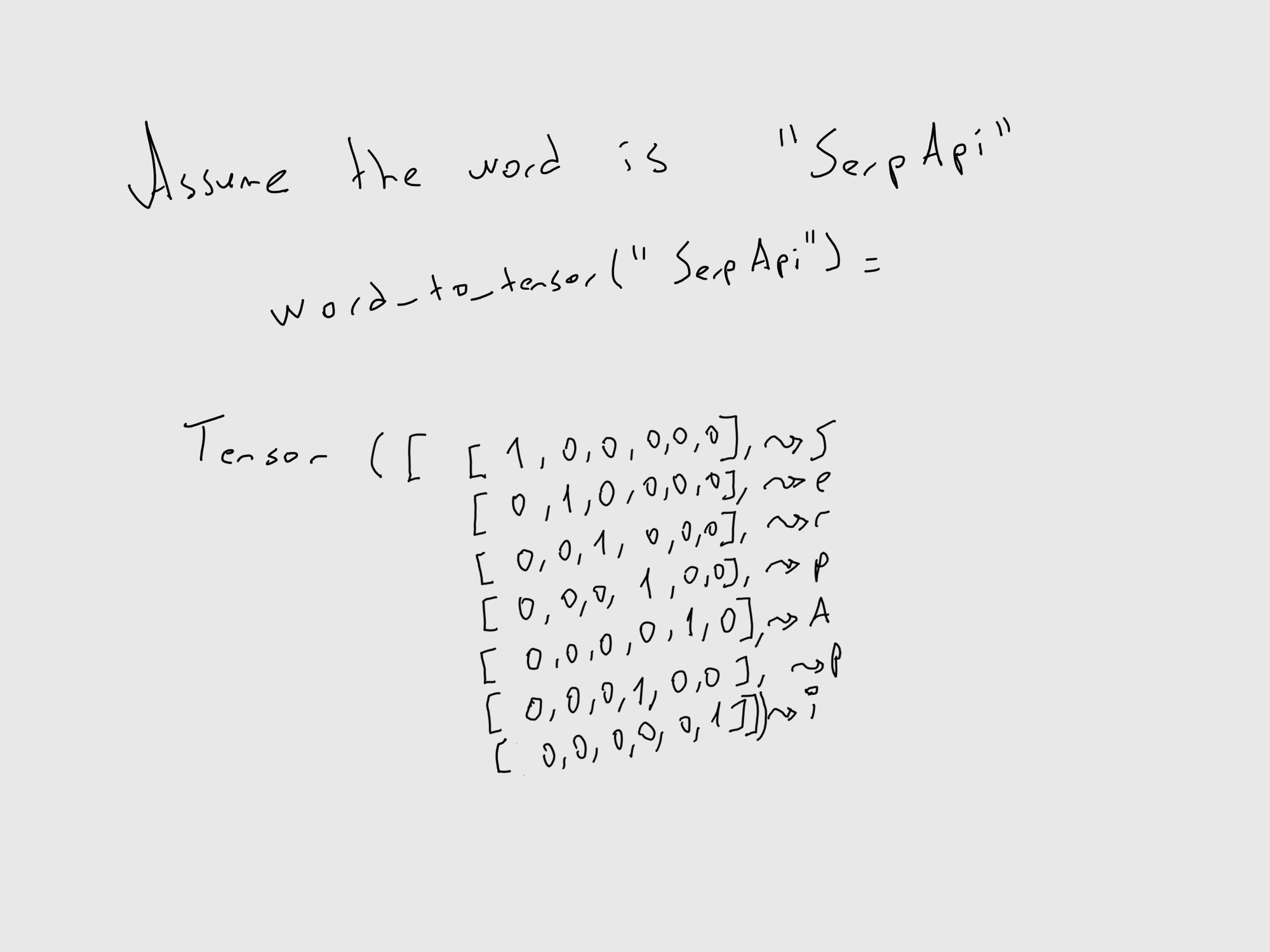
Creating The Model
Initialize our model within a class:
    def initialize input_size, hidden_size, output_size
      super()
      @hidden_size = hidden_size
      @i2h = Torch::NN::Linear.new(input_size + hidden_size, hidden_size)
      @i2o = Torch::NN::Linear.new(input_size + hidden_size, output_size)
      @softmax = Torch::NN::LogSoftmax.new(dim: 1)
    end
We feed the input_size which is …, hidden_size which is …, output_size which is … in our case.
@i2h represents Input to Hidden
@i2o represents Input to Output
@softmax here is the logarithm of softmax function in mathematics. Softmax is a probability distribution. In our case it’ll be the probability distribution of different keys within the SerpApi local results. Key with the highest probability will be given as an output.
Here's the visualization of the model:
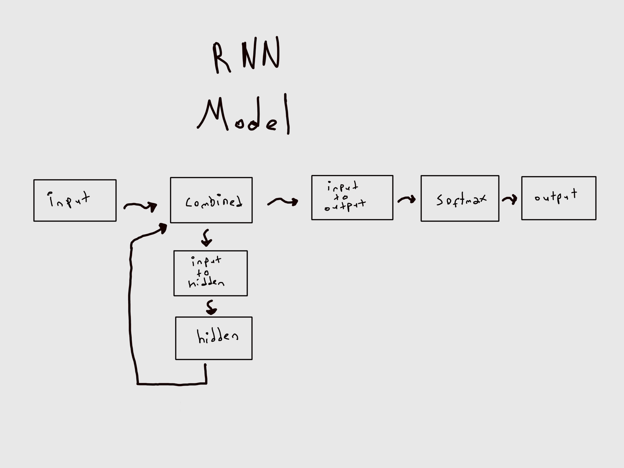
We need a way to forward the input data within the model.
    def forward input, hidden
      combined = Torch.cat( [input, hidden], dim:1)
      hidden = @i2h.call(combined)
      output = @i2o.call(combined)
      output = @softmax.call(output)
      return output, hidden
    end
We also need a way to initialize hidden layer zero tensor to be filled within the flow.
    def init_hidden
      Torch.zeros(1, @hidden_size)
    end
IV - Training The Model
There are necessary things we must define first. I’ll explain them in detail on next week’s blog post alongside some other details we will conclude. But simply put;
@n_epochs → Number of iterations a.k.a epochs
@print_every → At which rate do we want to print the current situation of the model on the terminal.
@plot_every → At which rate do we want to plot the progress to a graph.
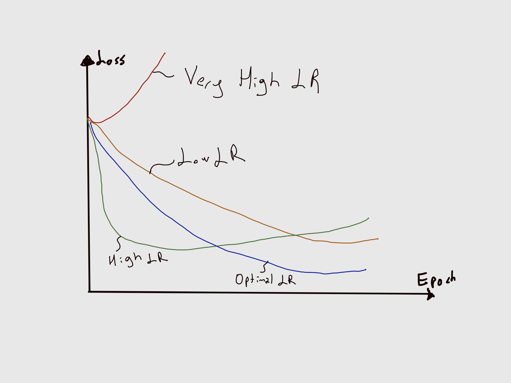
@learning_rate → Learning rate is responsible for the adjustment of weights within a machine learning model. In other words. It needs to be adjusted optimally.
Let me give a semantic example on learning rate:
Let’s assume you are teaching someone how to read. You taught the person the word Scraper, Skipper, Metamorphosis, and Pneumonoultramicroscopicsilicovolcanoconiosis (yes, a real word in English Language), alongside some other words. If you show Scraper, and ask him what this is;
-
If he tells you it is
Scraperit is a good learning rate.
It might tell you that is is something else until it learns. But you’ll recognize a sweet spot of failures, and you’ll still have a hope that this person will learn how to speak. -
If he tells you it is
Skipperit is a low learning rate.
This means the person is lost in details. Too many similar letters will mean same word to this person. -
If he tells you it is
Metamorphosis, it is a high learning rate.
The gap in differentiating words is too high for this person. This person is a deductive person now. -
If he tells you it is
Pneumonoultramicroscopicsilicovolcanoconiosis, it is a very high learning rate.
No way he’s gonna learn.
@n_categories → Number of categories, number of different keys in our case
@n_hidden → Size of Hidden layer. It could be tweaked to get different results. Also you may have different sets of hidden layers in front of each other with different sizes to get different results.
@net → Our Model
@optimizer → Stochiastic Gradient Descent function that is useful for adjusting weights between nodes to come up with an optimized model. Each iteration with positive outcome, match of inputted value, and outputted key in our case, will increase the model’s leniency to go from there given the input is similar, and each iteration with the negative outcome will decrease the model’s leniency to go from there given the input is dissimilar. With enough iteration, model will be optimized.
@criterion → Negative Log Likelihood is a function we use to determine the loss of a model. Loss is useful to observe the optimization of the model throughout different epochs.
  @n_epochs = 1000
  @print_every = 1000
  @plot_every = 1
  @learning_rate = 0.005
  @start = DateTime.now.to_f

  DataTools.new "ml/google/local_pack/data/local_pack_en-us.json"
  @all_letters, @n_letters = DataTools.declare_dictionary
  @data = DataTools.read_from_json
  @all_categories = @data.keys
  @n_categories = @data.keys.size
  @n_hidden = 128

  @net = GLocalNet.new(@n_letters, @n_hidden, @n_categories)
  @optimizer = Torch::Optim::SGD.new(@net.parameters, lr: @learning_rate)
  @criterion = Torch::NN::NLLLoss.new
  @current_loss = 0
  @all_losses = []
Now that we declared our necessary variables, let’s take a look at other functions we need.
This function is responsible for giving the highest possible output and its index within all categories:
  def self.category_from_output output
    top_n, top_i = Torch.topk(output.data, 1)
    category_i = top_i[0].item
    return @all_categories[category_i], category_i
  end
This function is responsible for picking a random value from an array:
  def self.random_choice arr
    max = arr.size - 1
    arr[rand(0..max)]
  end
This function is responsible for creating random training pairs. It picks a random category (key names in our case), picks a random word from that category, translates both of them into tensors and returns it. You can consider it as creating a random pop-quiz for the model.
  def self.random_training_pair
    category = random_choice(@all_categories)
    word = random_choice(@data[category])
    category_tensor = Torch.tensor([@all_categories.index(category)],dtype: :long)
    word_tensor = DataTools.word_to_tensor word
    return category, word, category_tensor, word_tensor
  end
This function is responsible for one epoch of training. It takes the category tensor and word tensor we created randomly, initiates a hidden layer, zeroes out the gradients (to keep it in buffers instead of overwriting), and then calls each letter tensor of the word tensor within the model. Output from that interaction is then used for measuring the loss of the epoch. Backward propagation is activated to accumulate buffers and then single optimization step is taken. Predicted output and the loss of the epoch are returned.
  def self.train category_tensor, word_tensor
    hidden = @net.init_hidden

    @net.zero_grad

    (0..word_tensor.size.first-1).each do |index|
      @output, hidden = @net.call(word_tensor[index], hidden)
    end

    loss = @criterion.call(@output, category_tensor)
    loss.backward
    @optimizer.step

    return @output, loss.data.item
  end
We also need a way to measure time for the overall process. It seems unimportant. But the training time of the model is truly one of the key features in scaling it.
  def self.time_since since
    now = DateTime.now.to_f
    seconds = now - since
    minutes = (seconds / 60).floor
    seconds = seconds - (minutes * 60)
    "#{minutes} minutes #{seconds} seconds"
  end
This next part is the brain of our training process where the data is trained. We train the model @n_epochs times. To calculate success rate, we’ll pass total_passed variable which’ll increase with each positive outcome.
At each epoch, we create a random training pair, train the model one time, get the current loss of our model, and check if the prediction is correct. Success rate will be created to measure the success of the model with the state of prediction. We’ll print the results at every @print_every. We’ll plot at every @plot_every to plot loss over epochs, and success rate over epochs.
  def self.iterate_epochs
    total_passed = 0
    success_rates = []
    (1..(@n_epochs+1)).each do |epoch|
      category, word, category_tensor, word_tensor = random_training_pair
      output, loss = train category_tensor, word_tensor
      @current_loss = @current_loss + loss

      guess, guess_i = category_from_output output
      state = guess == category ? "Passed" : "Failed"

      if state == "Passed"
        total_passed = total_passed + 1
      end

      success_rate = 100*(total_passed.to_f / epoch.to_f).round(6)

      if epoch % @print_every == 0
        puts "\n |Epoch: #{epoch} |\n "\
             "|Progress: %#{((epoch.to_f / @n_epochs.to_f).round(6))*100} |\n "\
             "|Time: #{time_since(@start)} |\n "\
             "|Loss: #{loss} |\n "\
             "|Guessed Value: #{word} |\n "\
             "|Guessed Field: #{guess} |\n "\
             "|Status: #{state} |\n "\
             "|Success Rate: %#{success_rate} |\n"\
             "----------------------------"
      end

      if epoch % @plot_every == 0
        @all_losses.append(@current_loss / @plot_every)
        success_rates.append(success_rate)
        @current_loss = 0
      end
    end

    plot_line_loss = Gruff::Line.new
    plot_line_loss.title = "Loss over #{@n_epochs} Epochs (At Every #{@plot_every} Epoch)"
    plot_line_loss.data :Loss, @all_losses
    plot_line_loss.write('ml/google/local_pack/predict_value/trained_models/rnn_value_predictor_loss.png')

    plot_line_sr = Gruff::Line.new
    plot_line_sr.title = "Succress Rate(%) over #{@n_epochs} Epochs (At Every #{@plot_every} Epoch)"
    plot_line_sr.data :Success, success_rates
    plot_line_sr.write('ml/google/local_pack/predict_value/trained_models/rnn_value_predictor_sr.png')
  end
We’ll also need to save the current state of the model to a file in order to use it:
  def self.save_model
    Torch.save(@net.state_dict, "ml/google/local_pack/predict_value/trained_models/rnn_value_predictor.pth")
  end
Example Results
Note that the results here are not conclusive. This is a model trained with 1000 epochs (fairly low). Thus, these results are only to show the functionality of the implementation.
Here is an example of a printed result:
 |Epoch: 1000 |
 |Progress: %100.0 |
 |Time: 0 minutes 5.2206950187683105 seconds |
 |Loss: 2.568265676498413 |
 |Guessed Value: Permanently closed |
 |Guessed Field: title |
 |Status: Failed |
 |Success Rate: %27.900000000000002 |
----------------------------
Here is an example of Success Rate over Epochs:
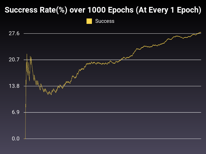
As you can see, with enough training, it seems like it can get to a state where it’ll predict the overwhelming majority of the inputs correctly.
Here is an example of Loss over Epochs:
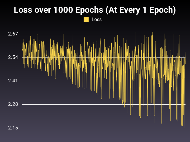
As you can see, low level of training is exposing oscillation within the loss. However the trend seems to be healthy.
Conclusion
I am grateful for the incredible support I received from the SerpApi team in crucial parts of the implementation. Also, I’m grateful for the creator and maintainer of gems we used to make this possible, and PyTorch for their incredible documentation.
Next week, I’ll go deeper into the explanations of the model, make some tweaks in it, and share the comparative results. Thanks for reading.
Acknowledgments:
- Gems Used:
torch.rb
torchtext-ruby
gruff - C++ Libraries Used:
LibTorch 1.10.2, Linux, CUDA 10.2, cxx11 ABI - Materials Repurposed From:
Blog Post
Documentation