 Ruby
Ruby
 Golang
 .Net
.Net
 MCP
MCP
 C++
C++

This week we'll talk about adjusting learning rate and yields of different optimizers and loss functions.
For those of you who aren't familiar with the dataset we use;
We are trying to distinguish different keys from SerpApi's Google Local Results Scraper API Results
Preliminary Results for Different Sets of Tweaks Graph (explained in detail below)
These results are not from the same training processes with the examples below. Numbers may vary but the average will be the same.
Let me show you how to load the model we created and how to call it for real work:
  def self.load word
    word_tensor = DataTools.word_to_tensor(word)
    net = GLocalNet.new(@n_letters, @n_hidden, @n_categories)
    net.load_state_dict(Torch.load("ml/google/local_pack/predict_value/trained_models/rnn_value_predictor.pth"))

    (0..word_tensor.size.first-1).each do |index|
      @predictions, hidden = net.call(word_tensor[index])
    end

    predictions = @predictions[0].to_a
    index = predictions.find_index predictions.max
    @all_categories[index]
  end
This is not a finalized version for the reasons I declared in blog post #1
Here are real examples of the model's predictions:
[1] pry(PredictValue)> load "Taco Bell"
=> "title"
[2] pry(PredictValue)> load "Quality coffee, chess & late hours are all draws at this relaxed, mural-decorated cafe."
=> "description"
[3] pry(PredictValue)> load "Georgetown, KY"
=> "address"
[4] pry(PredictValue)> load "Insurance agency"
=> "type"
[5] pry(PredictValue)> load "322"
=> "reviews"
[6] pry(PredictValue)> load "Closed ⋅ Opens 8AM Fri"
=> "hours"
[7] pry(PredictValue)> load "SerpApi"
=> "hours"
[8] pry(PredictValue)> load "$$"
=> "price"
[9] pry(PredictValue)> load "4.9"
=> "rating"
[10] pry(PredictValue)> load "+1 813-876-3354"
=> "rating"
As you can see, in its current state the output is giving interesting outputs like in the examples of "SerpApi" and "+1 813-876-3354". We are aiming to correct these mistakes and implement a highly efficient model in our parsers.
Let's dive deep into different learning rates and how they affect the model.
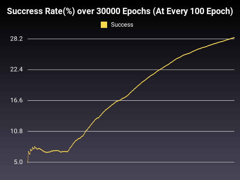
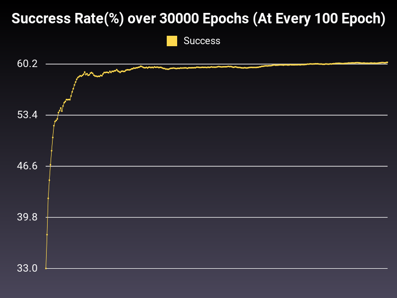
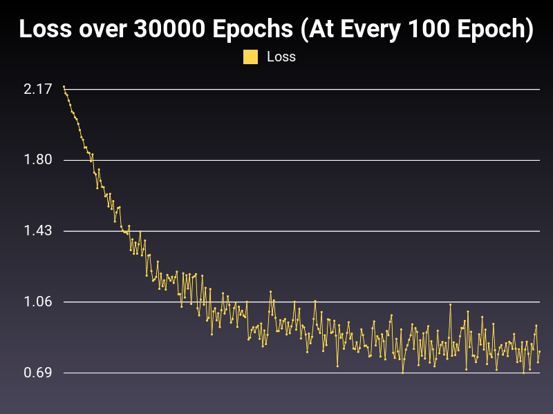
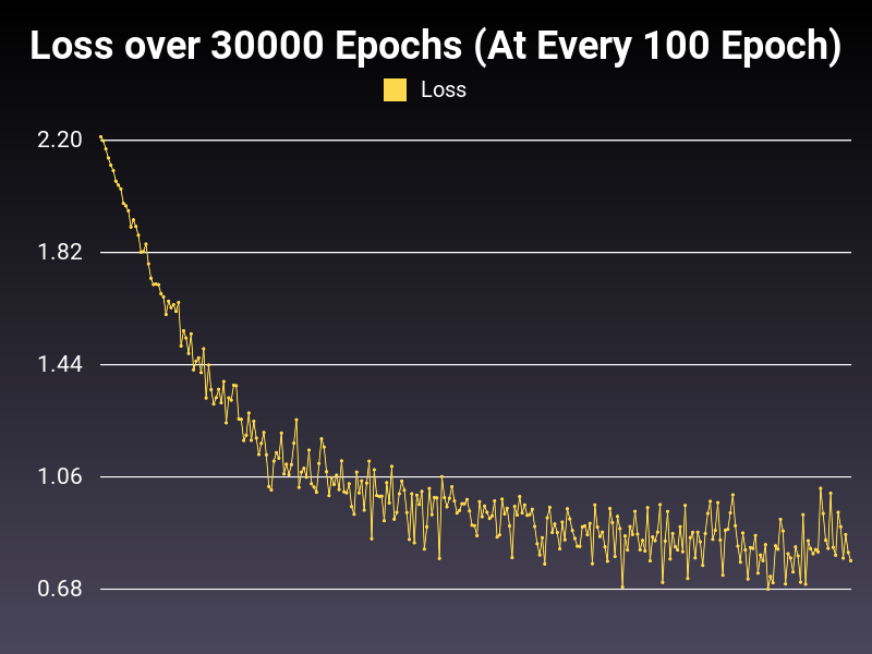
Example: Very High Learning Rate
Optimizer: SGD
Loss: NLLLoss
Hidden Layers: 128 (Only One)
Epochs: 30000
Runtime: 44 seconds (CUDA Enabled)
Learning Rate: 0.999 (Static)
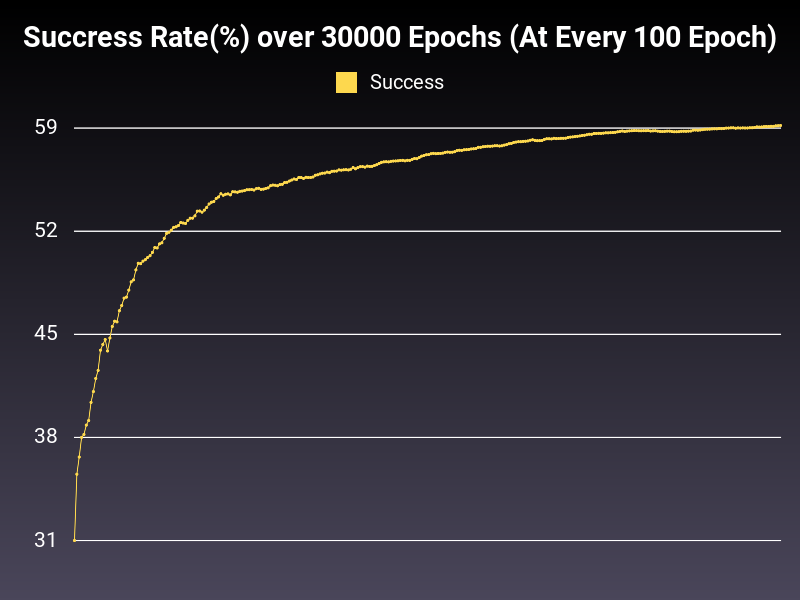
Accumulative Success: 57.07%
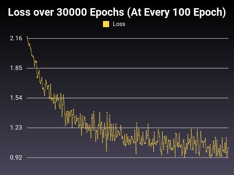
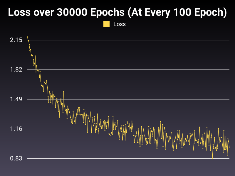
This is the problem with the very high learning rate. As you can see, the loss decreases drastically at first, and then goes up or stays same (as seen in the loss graph). This kind of learning rate is equivalent to studying on speed. You think you learn everything but you learn nothing. :)
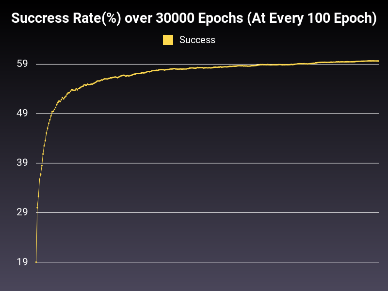
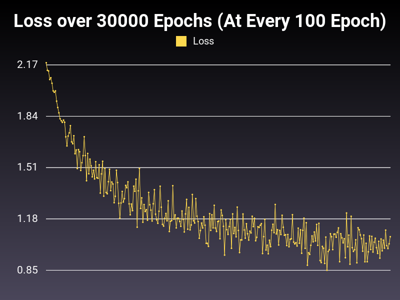
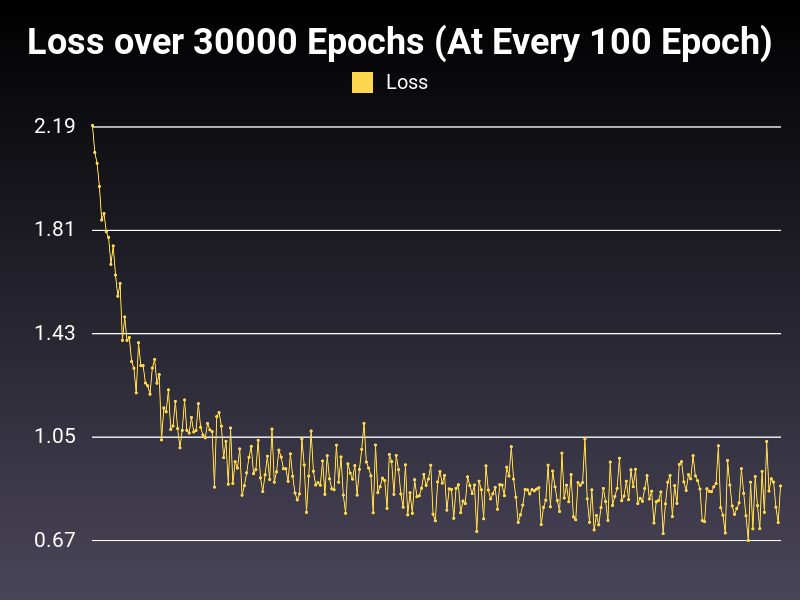
Example: Low Learning Rate
Optimizer: SGD
Loss: NLLLoss
Hidden Layers: 128 (Only One)
Epochs: 30000
Runtime: 46 seconds (CUDA Enabled)
Learning Rate: 0.001 (Static)
Accumulative Success: 51.9967%
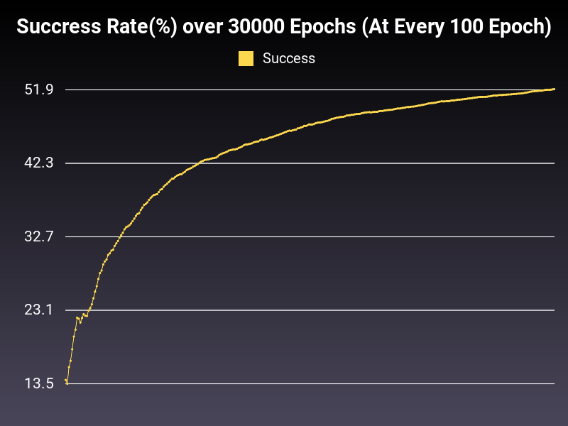
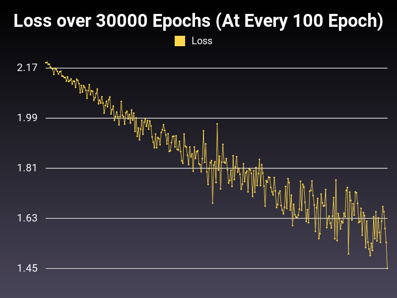
At low learning rate, we are able to bring down the loss, however the whole process is too slow for the 30000 epoch length. Also the oscillation in the range of loss is growing telescopically, creating inefficiencies in the trained model.
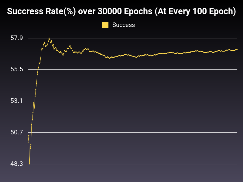
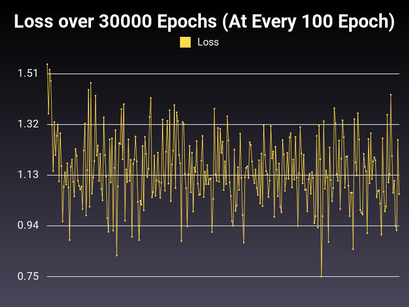
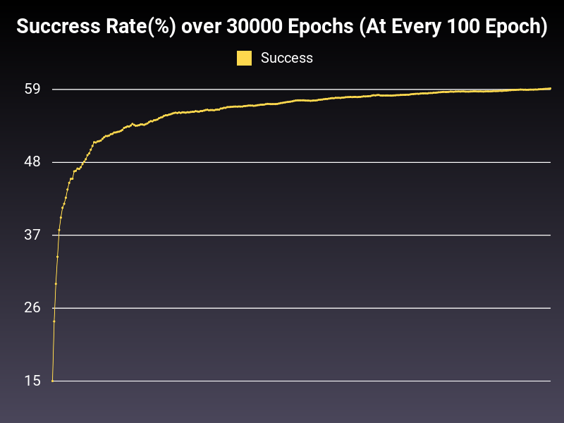
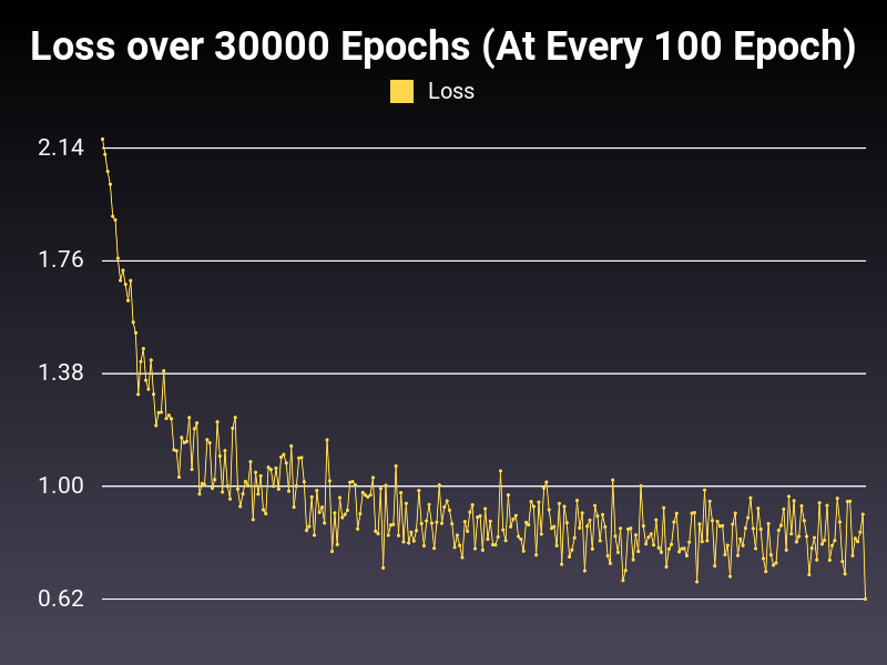
High Learning Rate
Optimizer: SGD
Loss: NLLLoss
Hidden Layers: 128 (Only One)
Epochs: 30000
Runtime: 44 seconds (CUDA Enabled)
Learning Rate: 0.1 (Static)
Accumulative Success: 59.753299999999996%
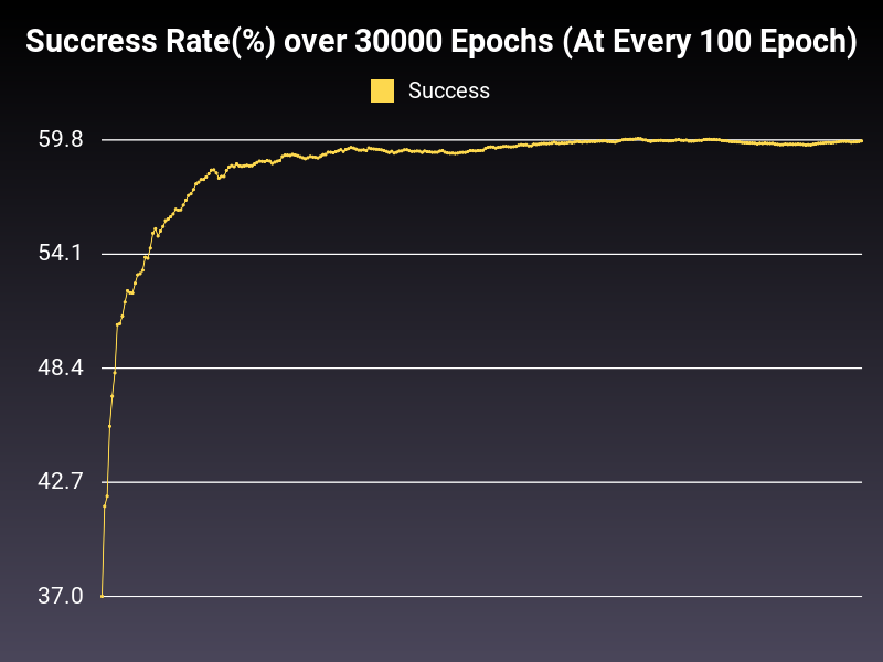
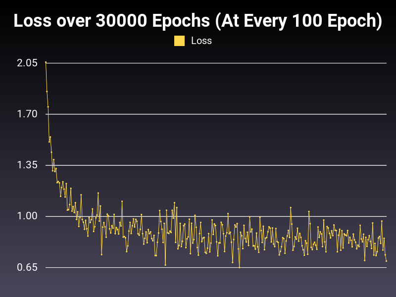
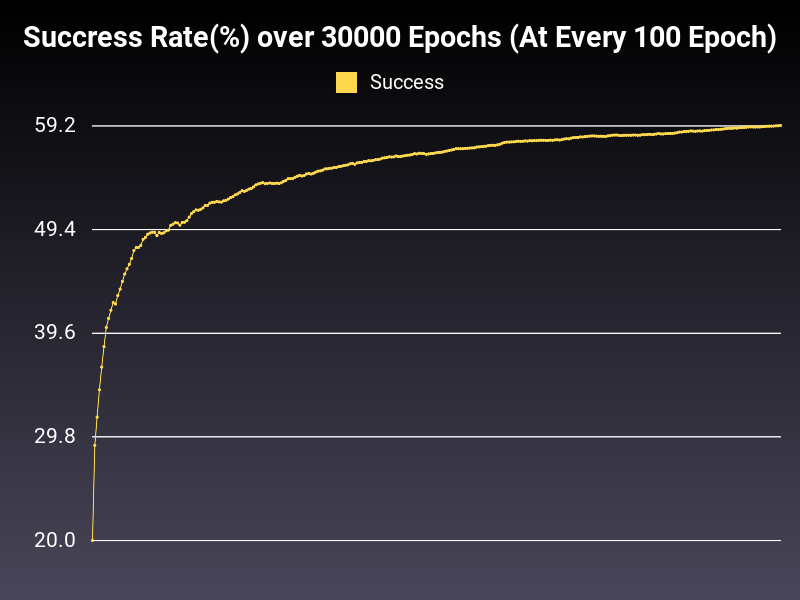
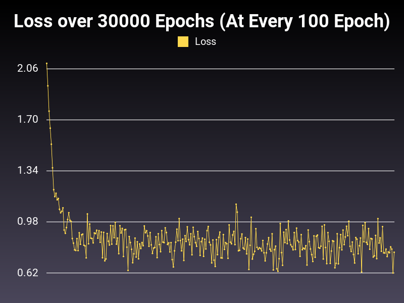
Learning Rate is too high. You can observe the loss function to get the impression. Roughly 60% seems to be the plateau value for this model with this optimizer and loss function, in this learning rate. So, what can we do to improve the situation? Let's decrease learning weight to a factor of 10 to observe the loss function again.
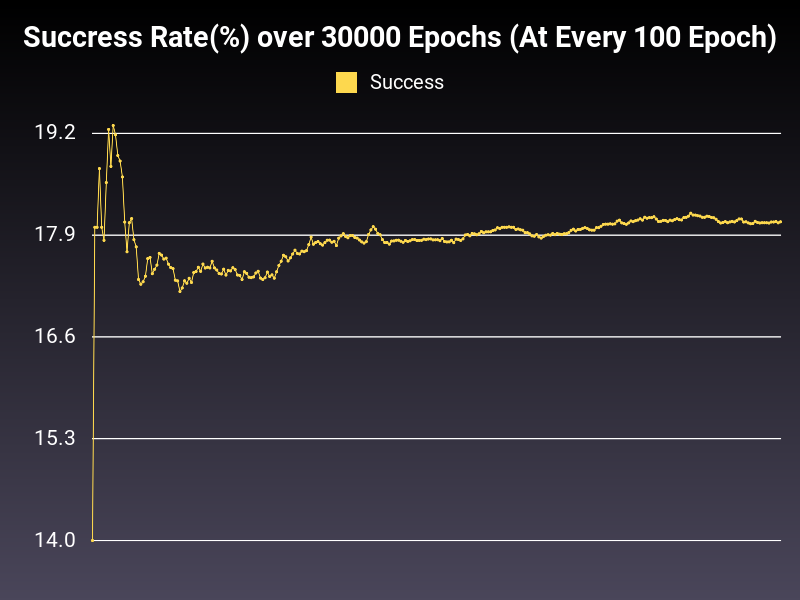
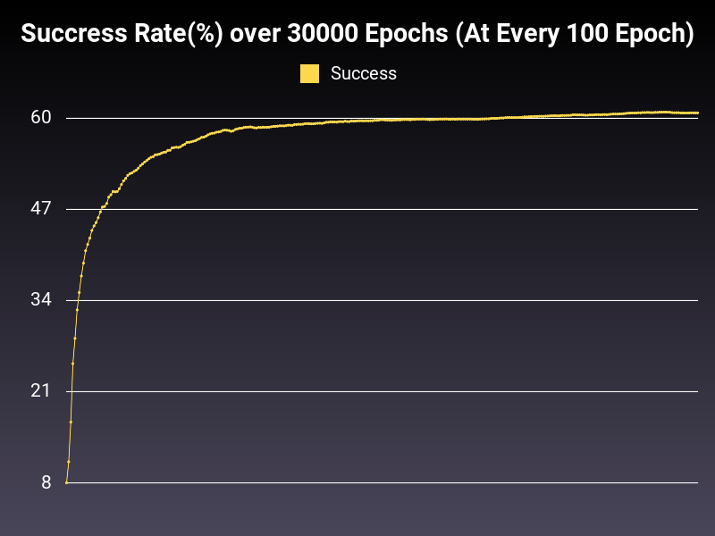
Good(ish) Learning Rate
Optimizer: SGD
Loss: NLLLoss
Hidden Layers: 128 (Only One)
Epochs: 30000
Runtime: 44 seconds (CUDA Enabled)
Learning Rate: 0.01 (Static)
Accumulative Success: 59.646699999999996%
This is more of a healthy trend line as you can see. However, oscillations are too big. There is also one more problem. The optimal learning rate might change from algorithm to algorithm. What can we do to expand the range of good learning rates without nitpicking too much? Let's explore this in the next part.
Customized Adaptive Learning Rate
First of all, we want our loss function to have a certain shape on the graph. Normally Pytorch has learning rate schedulers that are useful for adapting learning rates when the cumulative success rates are stagnating.
However, I wasn't able to find it in the library we are using. It gives us a good opportunity to come up with it our own way. Let's express the shape we want in polynomial form.
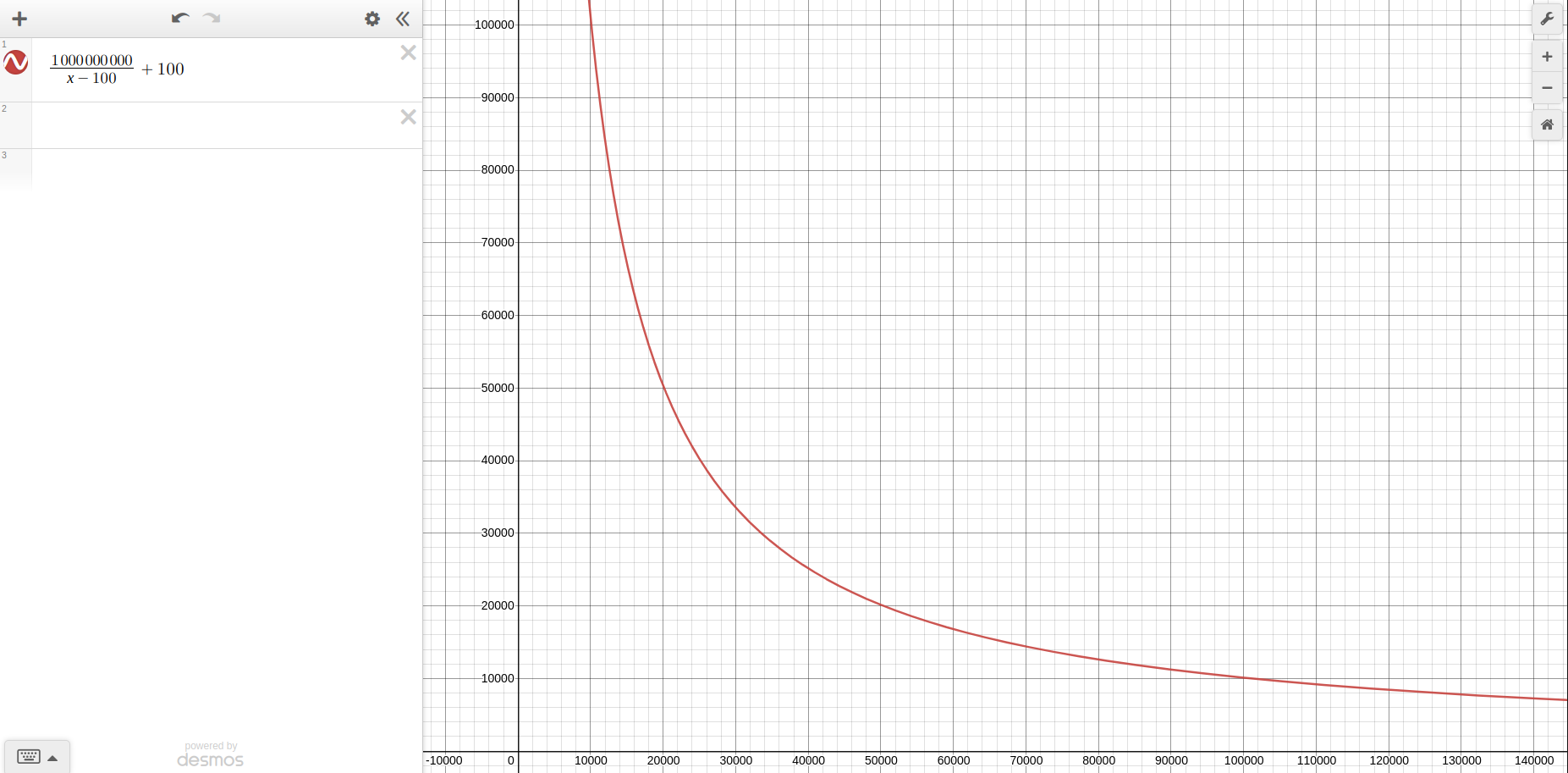
For those of you who want to have a closer look, I have used Desmos graphing calculator to come up with it. The functional command is \frac{1000000000}{x-100}+100.
This function gives us a good shape for the loss function. But how can we achieve general adjustment of the learning rate that will translate itself in the loss function?
I want the reader to take a closer look. As epoch (x-axis) goes to infinity, loss decreases at a certain rate. We can observe that change with taking the derivative of the ideal loss function we declared.
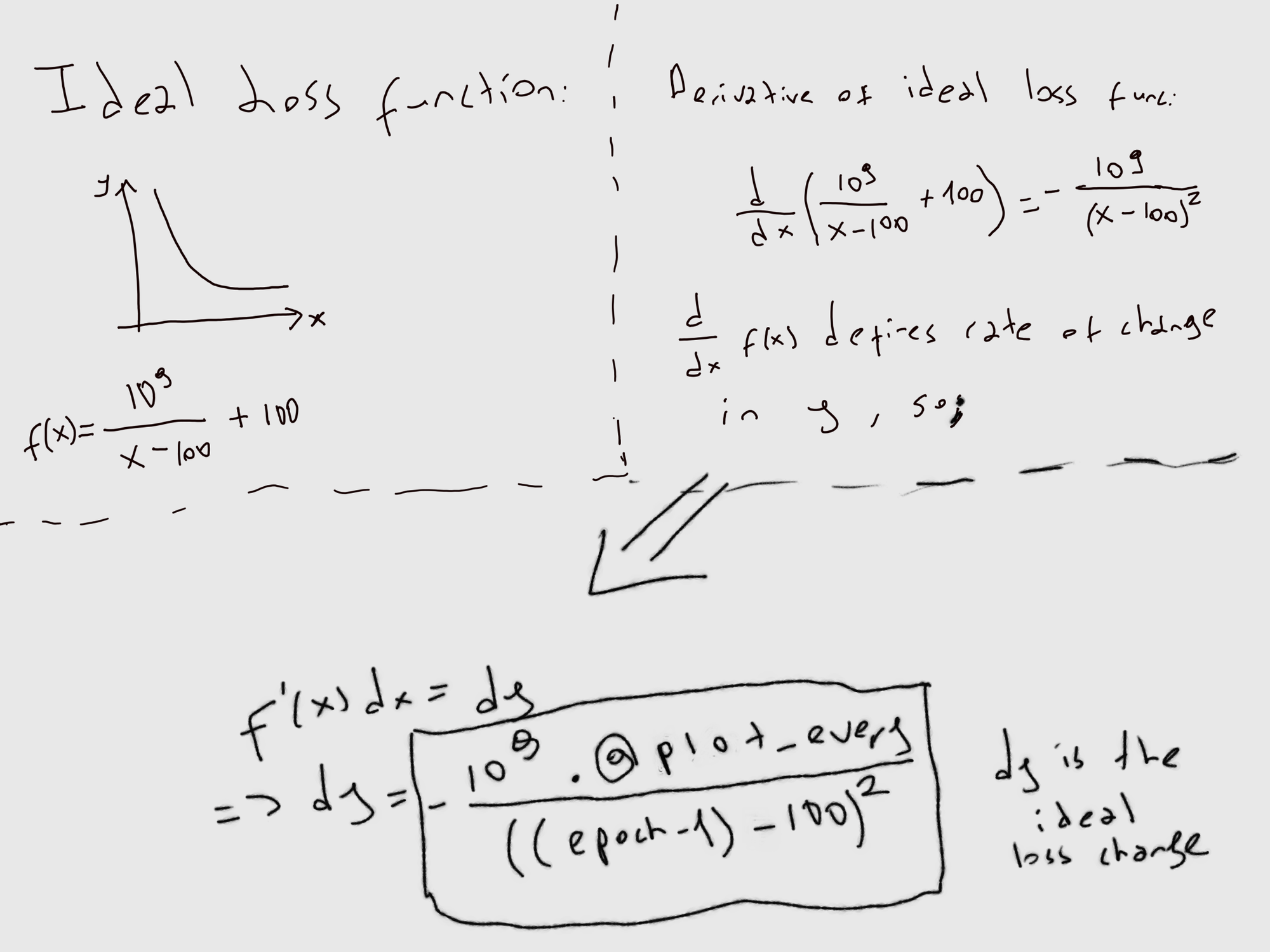
This is the change we want of loss each epoch. Let's declare it in our code:
  def self.ideal_loss_derivative x
    Float(-1000000000*@plot_every/((x-100)*(x-100)))
  end
Derivative of Ideal Loss Function
Now that we have a way to know what the change in loss should be, let's implement an algorithm that takes note of that and adjusts the learning rate:
  def self.adjust_lr(epoch)
    if @all_losses.size > 1
      low_training = (@all_losses[-1] - @all_losses[-2] > 0) || (@all_losses[-1] - @all_losses[-2] > ideal_loss_derivative(epoch-1))
      high_training = @all_losses[-1] - @all_losses[-2] < ideal_loss_derivative(epoch-1)

      if low_training
        @learning_rate = @learning_rate * 2
      elsif high_training
        @learning_rate= @learning_rate * 0.02
      end
    end
  end
Adjustment of Learning Rate
Let's break down what we did in here;
if @all_losses.size > 1We check for @all_losses size to be more than 1. For those of you who didn't read the previous blog post, @all_losses is an array where we collect all loss values at different epoch. The reason we start when it is at least 1 is simple, we want to be able to measure change. You need at least 2 elements to have change.
low_training = (@all_losses[-1] - @all_losses[-2] > 0) || (@all_losses[-1] - @all_losses[-2] > ideal_loss_derivative(epoch-1))If the change of loss on second to last element is greater than 0, we have a problem. Our loss is increasing instead of decreasing. So we can adjust the learning higher to resolve the problem. You can out the graphs for Low Learning Rate and Very High Learning Rate to see that increasing learning rate will do what we need to give our loss graph a shape.
high_training = @all_losses[-1] - @all_losses[-2] < ideal_loss_derivative(epoch-1)This is the way we will catch high learning rates for different epoch. Derivative of epoch-1 should give us the ideal change we should get. If the real change in loss is greater than what it should be we need to lower it to get a good learning rate.
      if low_training
        @learning_rate = @learning_rate * 2
      elsif high_training
        @learning_rate= @learning_rate * 0.2
      end
Without a precise function on how much to increase or decrease, let's apply fractional changes. The reason we are applying fractional changes is simple; to keep the learning rate above 0.
One more factor here to consider is that low training rate is more dangerous than high training rate. Simply put, low training rate will increase the loss function and will lead to deficiencies in the model whereas high training rate at different levels on a small scale will result in deficiency in optimization of the function. So, the aim is more important than the optimal state of the function.
Let's implement adjust_lr at where we expand @all_losses array:
      if epoch % @plot_every == 0
        @all_losses.append(@current_loss / @plot_every)
        adjust_lr(epoch-1)
        success_rates.append(success_rate)
        @current_loss = 0
      end
Of course, this will still yield bad results if the learning rate is too high or too low. But this function will change the definition of too high and too low and broaden our chances of getting a good learning rate, and provide smoother oscillation in long-range training.
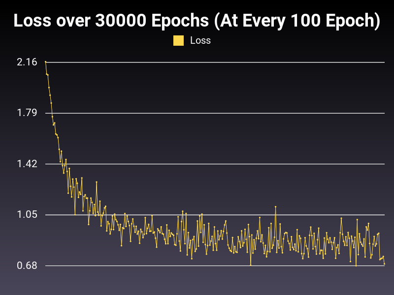
Trying Different Sets of Tweaks
Optimizer: SGD
Loss: CrossEntropyLoss
Hidden Layers: 128 (Only One)
Epochs: 30000
Runtime: 49 seconds (CUDA Enabled)
Learning Rate: 0.01 (Adaptive)
Accumulative Success: 59.1733%
Optimizer: SGD
Loss: NLLLoss
Hidden Layers: 128 (Only One)
Epochs: 30000
Runtime: 49 seconds (CUDA Enabled)
Learning Rate: 0.01 (Adaptive)
Accumulative Success: 59.1500%
Optimizer: Adadelta
Loss: CrossEntropyLoss
Hidden Layers: 128 (Only One)
Epochs: 30000
Runtime: 52 seconds (CUDA Enabled)
Learning Rate: 0.01 (Adaptive)
Accumulative Success: 28.4367%

Optimizer: Adadelta
Loss: CrossEntropyLoss
Hidden Layers: 128 (Only One)
Epochs: 30000
Runtime: 50 seconds (CUDA Enabled)
Learning Rate: 0.001 (Adaptive)
Accumulative Success: 18.07%

Optimizer: Adagrad
Loss: CrossEntropyLoss
Hidden Layers: 128 (Only One)
Epochs: 30000
Runtime: 50 seconds (CUDA Enabled)
Learning Rate: 0.01 (Adaptive)
Accumulative Success: 59.2433%

Optimizer: Adagrad
Loss: NLLLoss
Hidden Layers: 128 (Only One)
Epochs: 30000
Runtime: 48 seconds (CUDA Enabled)
Learning Rate: 0.01 (Adaptive)
Accumulative Success: 59.56%


Optimizer: Adam
Loss: CrossEntropyLoss
Hidden Layers: 128 (Only One)
Epochs: 30000
Runtime: 50 seconds (CUDA Enabled)
Learning Rate: 0.01 (Adaptive)
Accumulative Success: 60.4333%
Optimizer: Adam
Loss: CrossEntropyLoss
Hidden Layers: 128 (Only One)
Epochs: 30000
Runtime: 50 seconds (CUDA Enabled)
Learning Rate: 0.001 (Adaptive)
Accumulative Success: 60.9199%

Optimizer: Adam
Loss: NLLLoss
Hidden Layers: 128 (Only One)
Epochs: 30000
Runtime: 51 seconds (CUDA Enabled)
Learning Rate: 0.001 (Adaptive)
Accumulative Success: 60.7733%
Optimizer: Adamax
Loss: CrossEntropyLoss
Hidden Layers: 128 (Only One)
Epochs: 30000
Runtime: 54 seconds (CUDA Enabled)
Learning Rate: 0.01 (Adaptive)
Accumulative Success: 60.2733%

Optimizer: Adamax
Loss: NLLLoss
Hidden Layers: 128 (Only One)
Epochs: 30000
Runtime: 55 seconds (CUDA Enabled)
Learning Rate: 0.01 (Adaptive)
Accumulative Success: 60.19%

Optimizer: AdamW
Loss: CrossEntropy
Hidden Layers: 128 (Only One)
Epochs: 30000
Runtime: 55 seconds (CUDA Enabled)
Learning Rate: 0.01 (Adaptive)
Accumulative Success: 60.2167%

Conclusion
Preliminary results are not conclusive. However, there needs to be a change in the model itself to better iterate the yield of these optimizers (60% is not enough). Early tests show that one of the Adam functions will be better in giving results (healthy loss functions).
Next week, we will discuss the change we did. I am grateful to everyone in SerpApi who made this blog post possible. Thanks for reading and observing the findings. I hope they relay some understanding.